Introduction to Coding Theory

A practical example of error correction

How is it that a CD with so many scratches on it can still be played continuously with few audible errors? Why is it that a QR-code read incorrectly can still reveal the right information?

In other words, how can a CD-player or QR-code reader take a data stream with so many errors and correct most of them? This is where error correcting codes (a topic within Coding Theory) come into play.

Overview of error detection

In communications over noisy channels, like radio communications or the reading of a CD¹, the data is often not received as intended.

Suppose that I intend to send the following message to a friend through a noisy channel: Hi! ² This string is equivalent to the bits: 010010000110100100100001

However, my friend may receive this message as corrupted in ASCII. Flipped bits are marked in $\textcolor{red}{\verb|red|}$.

$$\textcolor{red}{1}10010\textcolor{red}{1}00110100\textcolor{red}{1}001 \textcolor{red}{1}0001 \longleftrightarrow \verb!Êi1!$$

Converting this transmitted message back to a string doesn’t even resemble a word! Over noisy mediums, error rates, like one-in-six ratio as in the example, are very common. Using check bits, however, we can devise of a simple way to detect an error (but not correct it).

Suppose that I send a message composed of three bits and a parity bit which is calculated by adding all the previous bits in the binary field \(\textbf{B} = \{0, 1\}\):

$$\verb|Message:| 011$$

$$\verb|Parity bit:| \textcolor{blue}{0 + 1 + 1 = 0} \verb| in | \textbf{B}$$

$$\verb|Final message:| 011\textcolor{blue}{0}$$

Such a scheme can detect only one error: Suppose that the message \(0100\) is received, then the receiver can perform a simple calculation to see that the number of \(1\)s in the first three bits is congruent to the parity bit in B. However, this particular scheme cannot detect two errors because the parity bit would not help in detecting an error³. The recipient of the data can only ask for a re-transmission in this scheme, an expensive and sometimes infeasible task.

With certain modifications, augmentations, and more complex calculations, schemes based solely on parity bits can detect a great deal of errors. Generally, the information rate for parity bit schemes is \(R:=\frac{n - 1}{n}\) where \(n\) is the length of the message⁴. However, this high information rate comes at the cost of not detecting a great deal of possible errors. These types of error-detecting schemes are widely implemented in ISBN numbers, bar-code scanners, and other noise-prone applications where re-scanning is a viable option.

Overview of error correction

In some situations, like reading a CD or in QR codes, detecting an error is simply not a viable choice as a corrupted bit cannot just be labeled as incorrect and subsequently discarded as the information may be vital. Here, error correction is important.

A simple error correction scheme is to simply append multiple copies of the original message and transmit it. For example, I can encode a message \(011\) as \(011, 011, 011\) and transmit \(011011011\). Then if a friend receives

\(011\textcolor{red}{10}1011 = 011, \textcolor{red}{10}1, 011\) he/she can take the majority-occurring message \((011)\) as the actual message and use it. Here the error correction and detection scheme corrects two errors but at the expense of more transmitted data. The information rate for such a scheme is \(R = \frac{1}{3}\), a very inefficient mechanism.

Defining Coding Theory

Coding Theory deals with the creation and analysis of efficient error-correction schemes to ensure that messages transmitted over noisy channels are properly received.

Further, Coding Theory aims to find the optimal balance of effectiveness and efficiency of error-correcting codes in various applications. In other words, Coding Theory aims to balance a high information rate with a high error correction rate. A message is

Finally, I include a useful graphic which outlines the procedure of error correction across noisy channels. A message is encoded into a codeword, transmitted across a noisy channel, and then decoded and corrected by the recipient.

[NoisyCommunication]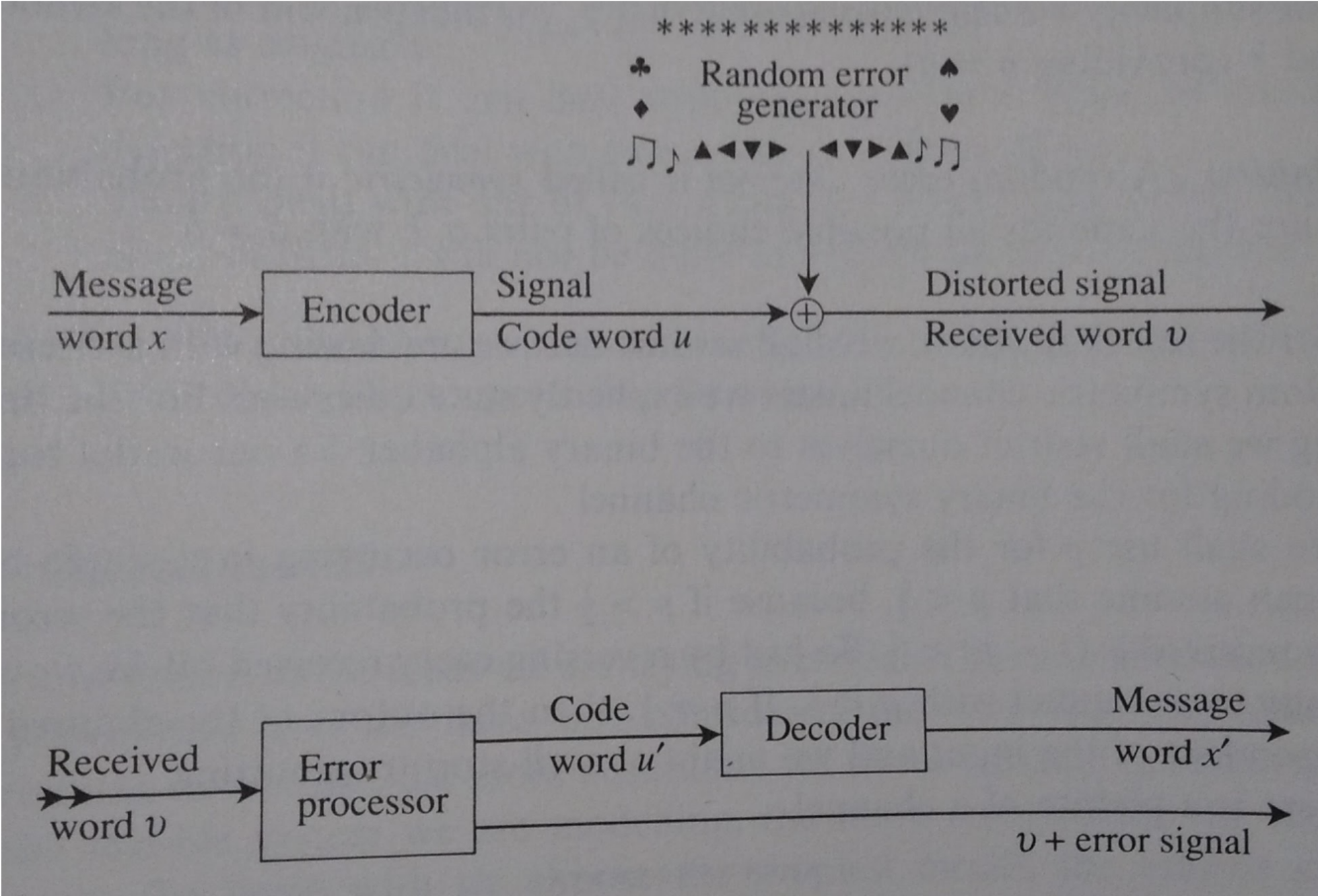

In this paper, I hope to effectively outline the use of Bose-Chaudhuri-Hocquenghem (BCH) codes which form a class of cyclic error-correcting codes constructed in finite fields.

Preliminaries to and definitions for discussing BCH codes ========================================

In the examples used in this paper, I will discuss the Galois field containing 16 elements notated as \(\textbf{GF}(16)\).

Code words and Hamming distances

Let’s first define some key words and concepts:

If \(A\) is an alphabet (containing \(q\) symbols), then an A-word with length \(n\) is denoted as \(A^n\) meaning that it contains \(n\) elements from \(A\). For example, in the set of alphabetic characters \(A = \{a, b, \cdots, z\}\), the A-word \(\verb|"hello"|\) is denoted as \(A^5\).

An \((n, m)\)-block code \(C\) over the alphabet \(A\) of size \(q\) contains exactly \(q^m\) code words in \(A^n\). The set of \(q^m\) elements in \(A^n\) consists of all the code words for a message of length \(n\) in the alphabet \(A\).

We will see that the field of code words defined in finite fields have special properties that would allow us to recover a corrupted message \(m\). In order encode some message \(m\), we use a bijective⁵ encoder \(E\) to map some \(m \in A^m\) to the set of code words \(C\) which have special properties as we will see.

We indulge in one more definition:

The Hamming distance

between two code words in \(u = (u_1, \ldots, u_n) \in A\) and \(v = (v_1, \ldots, v_n) \in A\) is a measure of how much \(u\) and \(v\) differ⁶. This distance is defined as the number of positions \(i\) where \(u_i \neq v_i\). In other words, the Hamming distance is a measure of how different two words are. For example, the distance between the vectors \(\verb|hello|\) and \(\verb|hi___|\) in the alphabet set \(A\) is 4 because the two vectors differ in value in four analougous locations.

Similarly, the minimum distance of the set \(C\) is smallest Hamming distance between any distinct pair of vectors in \(C\). The minimum distance is thus a measure of how “close” any two words are in a set of code words; the lower the minimum distance, the closer two words in the set \(C\) are. A code with a minimum Hamming distance of \(d\) can correct up to \(d-1\) errors in a code word. Usually, the set of code words \(C\) is designed to have a minimum Hamming distance

In error-correction schemes, when receiving a message vector in a noisy channel, say \(t = (t_1, \ldots, t_n)\), we are looking in the set of possible code words \(C\) to see what vector \(v\) in \(C\) has the smallest Hamming distance to \(t\). Then, this vector \(v\) is likely to be our intended message vector. In other words, we are trying to see what the message \(t\) is most likely trying to represent from \(C\).

Finite/Galois Fields

Alphabets used in error-correction schemes are usually constrained to \(256\) bits because they can represent all the common characters used in electronic communications. This leads to using a finite field of \(256\) elements. Here, we give a more formal definition of finite fields.

The finite field \(\mathbb{F}_q\) contains \(q\) elements and the standard arithmetic⁷ is constrained to this set of \(q\) elements. \(\mathbb{F}\) can also be considered a ring so \(\mathbb{F}[x]\) is the set of polynomials over \(\mathbb{F}\). Arithmetic in \(\mathbb{F}_n[x]\) can performed under a polynomial modulo and is denoted as \(\mathbb{F}_n[x]/f(x)\) for some irreducible⁸ polynomial \(f(x)\) that divides \((x^n - 1)\).

For the purposes of this paper, we will consider four bits as a single unit to deal with burst errors which tend to corrupt short and continuous segments of a code. As such, we will want to consider fields of size \(2^4 = 16\) as there are two elements in the alphabet \(\mathbb{B} = \{0, 1\}\) and the code word has length \(4\). As such, our finite field will can be denoted as \(\mathbb{B}_4[x]/f(x) = \textbf{GF}(16)\).

We cannot use integers in our construction of our finite field as they do not satisfy the cancellation law⁹ under non-prime modulo. So, we must use polynomials because they satisfy the required arithmetic properties.

Polynomials in finite fields

Because our field is \(\mathbb{B}_4[x]\), we are constrained to using binary coefficients to describe our polynomials. From binary strings, we can easily represent polynomials in \(\pmod{16}\). For example: \(1 \times x^3 + 0 \times x^2 + 1 \times x^1 + 1 \times x^0 = x^3 + x + 1 \leftrightarrow 1011 \leftrightarrow 8 + 0 + 4 + 1 = 13\) Polynomial addition is the same as addition over \(\mathbb{B}\). For example, adding \(101 \leftrightarrow x^2 + 1\) and \(011 \leftrightarrow x + 1\) results in \(x^2 + x + (1 + 1) = x^2 + x \leftrightarrow 110\). You may, correctly note that this resembles an \(\verb|XOR|\) operation.

Polynomial multiplication is a little more involved and is covered in more detail soon.

Constructing a finite field with polynomials

We have seen that using composite numbers \(c\) in \(\mathbb{Z}/c\mathbb{Z}\) does not allow the set of integers \(\{0, \ldots, c-1\}\) to satisfy the cancellation law. Using numbers like 16 as the modulus for a finite field leads to results like \(4 \times 4 \equiv 16 \equiv 0\) which are troubling to finite fields. This is why we chose polynomials as our arithmetic “basis” for math in the finite field \(\mathbb{B}_4[x]/f(x)\).

Thus, for the construction of a finite field, other than \(\mathbb{F}_p\) for a prime \(p\), we must choose polynomials \(g(x)\) in \(\mathbb{F}_n[x]\) that are irreducible¹⁰ factors of \(x^n - 1\). One such factor of \(x^{16} - 1\) in GF(16) is \(g(x) = x^4 + x^3 + 1\) and will be used to construct a finite field below.

To construct the finite field \(\textbf{GF}(16)\) using our generator polynomial \(x^4 + x^3 + 1\), we must first observe that \(x^4 = x^3 + 1\) because coefficients of \(-1 \equiv 1\) in \(\mathbb{B}\). The finite field itself is found by each possible binary polynomial under degree of \(4\). The set of possible polynomials each representing an integer from \(0\) to \(16\) is listed below in abbreviated form¹¹.

 **Polynomial**      **Binary**   **Decimal**   --------------------- ------------ -------------
        0               0000           0
        1               0001           1
       $$x$$              0010           2
     $$x + 1$$            0011           3
      $$x^2$$             0100           4
    $$x^2 + 1$$           0101           5
  $$x^2 + x + 1$$         0111           6
    $$\cdots$$          $$\cdots$$     $$\cdots$$    $$x^3 + x^2 + x + 1$$      1111          15

Now, to actually construct the field, we compute a table by multiplying the polynomial representations of each binary number from the rows and columns together to form a cell:

          0001   0010          0100   $$\cdots$$     1111   ---------- ------ ------ ------ ------ ---------- ----------
 0001     0001   0010   0011   0100   $$\cdots$$     1111
                 0100          1000   $$\cdots$$     0111
 0011                   0101   1100   $$\cdots$$     1000
 0100                          1001   $$\cdots$$     1110    $$\cdots$$                               $$\ddots$$   $$\vdots$$
 1111                                              0011

For example, to compute \(2 \times 3 \leftrightarrow 0010 \times 0011\), we compute the product of the polynomials: \((x) \times (x + 1) = x^2 + x \equiv x^2 + x \leftrightarrow \textcolor{green}{\textbf{0110}}\) For another example, we compute \(1111 \times 0010\): \((x^3 + x^2 + x + 1) \times (x) = x^4 + x^3 + x^2 + x\) Using the fact that \(x^4 = x^3 + 1\) in \(\mathbb{B}\) we must further reduce this polynomial so it exists in \(\textbf{GF}(16)\) because \(x^4\) is not defined in the field. \(\begin{aligned} x^4 + x^3 + x^2 + x &= (x^3 + 1) + x^3 + x^2 + x\\ &= (x^3 + x^3) + x^2 + x + 1 \\ &= x^2 + x + 1 \leftrightarrow 0111 \text{ } \checkmark \\ \end{aligned}\) Below is a completed table (in base 10) based on the primitive, generator polynomial \(x^4 + x^3 + 1\) (Figure [mult]).

Primitive elements in GF(16) ——————————–

Similar to a primitive root for a prime number, a primitive element in a finite field can generate all elements of a field in some permutation. In other words, \(\alpha \in \textbf{GF}(n)\) is a primitive element if the set \(\{a^0, a^1, \ldots, a^{n-1}\}\) is a permutation of \(\{1, 2, \ldots, n - 1\}\).

For the field GF(16), \(\alpha = 2\) is a primitive element because all powers of \(\alpha\) up to \(15\) serve as a permutation of the set \(\{1, 2, \ldots, n - 1\}\). Using the multiplication table in Figure [mult], we can easily verify this fact.

Overview of BCH

To develop a BCH code, we use all of the knowledge we have outlined above. Given a binary message expressed as a polynomial called \(u(x)\), we can map it to an encoded code word \(c(x)\) that lies in the set of valid BCH code words¹². We then convert \(c(x)\) to binary and transmit across a noisy channel.

The receiver will then perform various polynomial operations, calculate syndromes (yet to be discussed), and linear algebra row-reduction to eventually calculate where the corrupted bits are.

Encoding in BCH

To illustrate the BCH encoding and decoding procedures, we will use the example of a triple-error correcting \((15, 5, 7)\)BCH code in the GF\((16)\) based on the primitive¹³ polynomial \(x^4 + x + 1\)¹⁴.

First, let us clarify what a \((15, 5, 7)\)BCH code is:

The \(15\) represents

the size of the binary message transmitted. The size of a message is limited by the size of the finite field we are using. In this case, we are using GF\((16)\) so the size of our message is limited to \(16 - 1 = 15\). This value for \(15\) is also directly related to the maximal power of a polynomial code word as we will soon see.

The \(5\) represents

the number of information bits that can be transmitted.

The \(7\) represents

the number of check bits needed to correct the \(3\) errors we expect to introduce to our \(15\) bit overall message. The designed minimum distance in this code is \(7\) which is a requirement to correct \(3\) errors¹⁵.

Primitive elements and minimal polynomials in GF(16)

Now, given a primitive element \(\alpha\), we can find various minimal polynomials¹⁶ \(\phi_j(x)\) for each power of \(\alpha\) given below.

                 Powers of $$\alpha$$                              Minimal polynomial   -------------------------------------------------------- ---------------------------------------
    $$\{\alpha, \alpha^2, \alpha^ 4, \alpha^8 \}$$              $$\phi_1(x) = x^4 + x + 1$$
  $$\{\alpha^3, \alpha^6, \alpha^9, \alpha^{12} \}$$      $$\phi_3(x) = x^4 + x^3 + x^2 + x + 1$$
            $$\{\alpha^5, \alpha^{10}\}$$                       $$\phi_5(x) = x^2 + x + 1$$    $$\{\alpha^7, \alpha^{11}, \alpha^{13}, \alpha^{14} \}$$        $$\phi_7(x) = x^4 + x^3 + 1$$

Note that each power \(i\) of \(\alpha\) (i.e. \(\alpha^i\)) is a multiple of the corresponding minimal polynomial function \(\phi_j(x)\).

Finding a generator polynomial g(x)

Now, we must construct our generator function \(g(x)\) that will aid in creating our BCH code word. We find \(g(x)\) as such (using our table above). We find the LCM of three minimal polynomials because we are trying to correct three errors. \(\begin{aligned} g(x) &= LCM\{\phi_1(x), \phi_3(x), \phi_5(x)\} \\ &= (x^4 + x + 1) (x^4 + x^3 + x^2 + x + 1) (x^2 + x + 1) \\ &= x^{10} + x^8 + x^5 + x^4 + x^2 + x + 1 \\ \end{aligned}\)

Now, we have finally established that the polynomial \(g(x) = x^{10} + x^8 + x^5 + x^4 + x^2 + x + 1\) can correct three errors in a \((15, \textbf{\underline{5}}, 7)\) BCH code.

Encoding our message into a codeword of BCH

Next, suppose that we would like to send a message \(m(x)\). We can express our **** message in equivalent forms: \(m: 10110 \leftrightarrow m(x) = 1\cdot x^4 + 0\cdot x^3 + 1\cdot x^2 + 1\cdot x^1 + 0\cdot x^0 = x^4 + x^2 + x\) Now, we must find our transmitted word \(t(x)\):

1. First, we find the parity bits polynomial \(b(x)\). So, we must find the residue of \(x^{10} \cdot m(x)\) in the GF\((16)\) based on the primitive polynomial \(x^4 + x + 1\).

   In this case, we operate under \(\pmod{g(x)}\). Our final expression is evaluated as such¹⁷:

   \[\begin{aligned} b(x) = x^{10} \cdot m(x) &= x^{10} \cdot (x^4 + x^2 + x) \\ &= x^{14} + x^{12} + x^{11}\\ &\equiv -2 x^9-x^8-2 x^6-2 x^5-x^4-x^3-x^2-x \pmod{g(x)} \\ &\equiv x^8 + x^4 + x^3 + x^2 + x \pmod{g(x)} \end{aligned}\]

2. Second, we find \(t(x)\) by adding \(m(x) \cdot x^{10}\) and \(b(x)\):

   \(\begin{aligned} t(x) &= m(x) \cdot x^{10} + b(x) \\ &= (x^4 + x^2 + x) \cdot x^{10} + (x^8 + x^4 + x^3 + x^2 + x) \\ &=x^{14} + x^{12} + x^{11} + x^8 + x^4 + x^3 + x^2 + x \\ & \leftrightarrow t: 101100100011110 \end{aligned}\) Now, suppose we have transmitted the code word \(t\). In transmission over a noisy channel, the error vector \(e: 001000001000001\) is introduced to the transmission \(t\). Adding the polynomials \(t(x)\) and \(e(x) = x^{12} + x^6 + 1\) we find the vector/polynomial \(r(x)\) received is¹⁸. \(\begin{aligned} r(x) &= t(x) + e(x) \\ &= (x^{14} + x^{12} + x^{11} + x^8 + x^4 + x^3 + x^2 + x) + (x^{12} + x^6 + 1) \\ &= x^{14} + x^{11} + x^8 + x^6 + x^4 + x^3 + x^2 + x + 1 \\ & \leftrightarrow 100100101011111 \\ \end{aligned}\)

   Summarizing our results thus far

   The transmitted, error, and received vectors are included below for convenience ( and resemble flipped bits):

   ---

          $$t$$            101100100011110
   

   \(\textcolor{red}{e}\)
   \(r\) 101001001111

   ---

Decoding and error correction in BCH

Structure of BCH cyclic codes

Before delving in the decoding and error correction of our sample BCH code, we should discuss the structure of these codes.

BCH codes are cyclic codes that are constructed by specifying the zeros of their generator polynomials (\(g(x)\) in our case). BCH generator polynomials have a special property that the polynomial’s roots are consecutive. Namely, the generator polynomial \(g(x)\) has \(2t_d\) consecutive roots \(\alpha^b, \alpha^{b+1}, \ldots, \alpha^{b + 2t_d - 1}\) where \(\alpha\) is a primitive element and \(t_d\) is the number errors that the BCH code can correct. This fact arises from the fact that BCH codes have a minimum designed minimum Hamming distance of \(2t_d + 1\).

Decoding BCH codes

To decode binary codes in BCH, we must use the elements of GF(16) to number the positions of a codeword. For a vector \(r\) or length \(n\), the numbering is illustrated as such:

values     $$r_o$$    $$r_1$$     $$\ldots$$     $$r_{n-1}$$

positions \(1\) \(\alpha\) \(\ldots\) \(\alpha^{n-1}\)

In GF(16) arithmetic, we can find the positions of the errors (bottom row of the table above) by solving a set of equations. These equations can be found from the error polynomial \(e(x)\) and the zeros of the code \(a^j\) for \(b \leq j \leq b + 2t_d - 1\).

Let \(r(x) = m(x) + e(x)\) represent the polynomial associated with a received codeword where the error polynomial is defined as \(e(x) = e_{j_i}x^{j_i} + \cdots + e_{j_v}x^{j_v}\) for \(v \leq t_d\) is the number of errors. The sets \(\{e_{j_1}, \ldots, e_{j_v}\}\) and \(\{\alpha^{j_1}, \ldots, \alpha^{j_v}\) are known as the error values and error positions respectively where \(e_j \in \mathbb{B} = \{0, 1\}\) for binary BCH codes and \(\alpha \in \textbf{GF}(16)\)¹⁹.

We can then calculate syndrome values as such by evaluating \(r(x)\) at each of the zeros of the code (which we have established to be powers of \(\alpha\)):

Then we can define our error locater polynomial as: \(\sigma(x) = \prod_{l=1}^{v} (1 + a^{j_l}x) = 1 + \sigma_1x + \cdots + \sigma_v x^v\)

Finally, the roots of this polynomial are equivalent to the roots of the inverses of the error locations in \(r(x)\). Finally, we can make the following relation between the coefficients of \(\sigma(x)\) and the syndromes as such.

Solving this matrix for the \(\sigma\) vector will give us the coefficients in the error locater polynomial \(\sigma(x)\). This matrix is also referred to as the key equation. There are multiple algorithms to solve for the \(\sigma\) vector:

a

Euclidean algorithm

Berlekamp-Massey algorithm (BMA)

The Peterson-–Gorenstein–-Zierler (PGZ) decoder

In this example, we will use the PGZ decoder.

Continuing our example…

Now, the binary message \(r: 10\textcolor{red}{0}10010\textcolor{red}{1}01111\textcolor{red}{1}\) is received and the recipient proceeds to determine the and correct the errors.

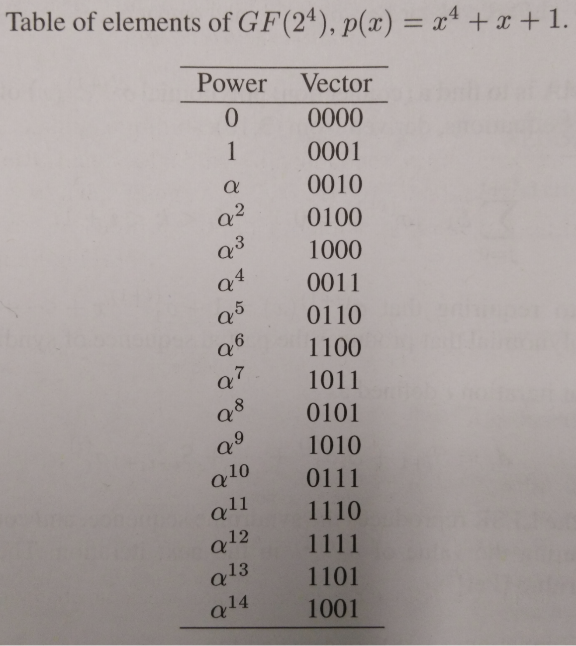
The recipient must first calculate values known as syndromes by evaluating the recevied message polynomial \(r(x)\) for corresponding powers of the primitive element \(\alpha \in \textbf{GF}(16)\). The syndromes are calculated as such using the Power/Vector table provided in the Appendix:²⁰

Restating our findings:

Now, knowing the six syndrome values for the received message \(r\), we can proceed to use the Peterson–-Gorenstein–-Zierler algorithm to find the error locations of \(r\).

The Peterson-–Gorenstein–-Zierler (PGZ) decoder

The decoding problem with BCH is that the number of errors in a message \(r\) are unknown to a recipient.

The PGZ process begins by filling the matrix from prior with values that we know for \(v = 3\) representing the three number of errors we can correct:

Because the \(\sigma_i\) values below are the inverses of the error positions, we must find the solution to the matrix equation:

Finding a solution for the \(\sigma\) vector is equivalent to seeing if \(\left( \begin{array}{ccc} \alpha & \alpha^2 & \alpha^8 \\ \alpha^2 & \alpha^8 & \alpha^4 \\ \alpha^8 & \alpha^4 & 1 \\ \end{array} \right)\) is invertible. This is equivalent to the matrix having a non-zero determinant²¹.

Let us calculate this determinant:

Because the determinant of the matrix is non-zero, then the matrix equation

must have a solution for the \(\sigma\) vector. Through a multitude of methods, we can solve the matrix equation above for the \(\sigma\) vector. Any such valid calculation (involving inverses and matrix multiplication²² reveals the following vector:

It follows by our definition of the error locater polynomial that: \(\sigma(x) = \alpha^3 x^3 + \alpha^7 x^2 + \alpha x + 1\) This polynomial also factors in \(\textbf{GF}(16)\) with our primitive root \(\alpha\)²³ as such. \(\sigma(x) = (1+x)(1+\alpha^6)(1+\alpha^{12}x)\) This factorization allows us to see that the factors of this equation are \(1=\alpha^0, \alpha^9 = \alpha^{-6}\), and \(\alpha^3 = \alpha^{-12}\).

These powers of these inverses in fact correspond to error positions as such:

Root of \(\sigma(x)\) Inverse of root Negative of power Corresponding polynomial

       $$1$$             $$\alpha^0$$             $$0$$                    $$1$$
   $$\alpha^9$$         $$\alpha^{-6}$$           $$6$$                   $$x^6$$
   $$\alpha^3$$        $$\alpha^{-12}$$          $$12$$                  $$x^{12}$$

These terms are identical to the terms of the error polynomial \(e(x) = x^{12} + x^6 + 1\). To the receiver, who has just calculated this error polynomial for him/herself, the corresponding bits (12th, 6th, and 1st) are flipped²⁴ to recover the original message. The final step is completed by adding the two vectors/polynomials²⁵.

     Received $$r(x)$$         $$x^{14} + x^{11} + x^8 + x^6 + x^4 + x^3 + x^2 + x + 1$$
   **** $$e(x)$$ vector                           $$x^{12} + x^6+ 1$$

Original \(m(x)\) message \(t\) \(x^{14} + x^{12} + x^{11} + x^8 + x^4 + x^3 + x^2 + x\)

Summarizing our results

      Received $$r$$ vector           101001001111
        **** $$e$$ vector            001000001000001

Computed original \(m\) message \(t\) 101001001111

Now, the original message is the first five bits 10110. This message has been recovered, without error, due to this implementation of a BCH code. The information rate for this \((15, 5, 7)\)BCH code is

The decoding and error correction segment of this algorithm is essentially a way to find the BCH code word that has a minimum distance to the received vector \(r\). This code word (in the set of BCH code words) then must be the intended sent code word before an error acted upon it.

Conclusion

Through our example of a BCH code, we required that calculations take place in \(\textbf{GF}(16)\) and with codewords expressed in binomial coefficients in \(\mathbb{B}\). Reed-Solomon codes drop this last condition and allow the terms our message to be expressed in \(\textbf{GF}(16)\). As such, Reed-Solomon codes are considered a special subset of BCH codes. Such Reed-Solomon codes are used in most CD players, QR-code readers, and even in communication between NASA and it Voyager deep-space probes.

For example, our example of a 5-bit message (\(10110\))is not longer constrained to 0s and 1s. Now, we can send messages in the set GF(16). Conveniently, data in computers is commonly represented in hex-code (in base 16) so we can send a string of data with 16 times more information!

In this paper, we have discussed Coding Theory, finite/Galois fields (and their various properties), polynomial arithmetic in these fields, and a complete example of BCH codes.

Appendix

Power/Vector table

References